
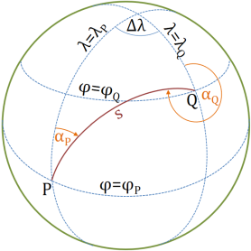
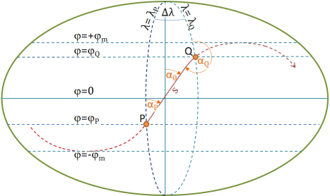
Es gibt sechs ausgezeichnete Kurven, die zwei gegebene Punkte P und Q auf einem Ellipsoid verbinden können:
Eine geodätische Linie ist die kürzeste Kurve innerhalb einer Fläche, die zwei gegebene Punkte verbindet. In unserem Fall ist die Fläche immer ein Rotationsellipsoid, welches die Erdfigur approximiert.
Es gibt im Wesentlichen 6 Größen, die den Verlauf einer geodätischen Linie PQ beschreiben:
Daneben haben noch folgende Größen eine gewisse Bedeutung:
Statt der ellipsoidischen Breiten φ können für P,Q,m auch die reduzierten Breiten β oder die geozentrischen Breiten ψ verwendet werden.
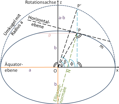
| P | Punkt auf dem Ellipsoid |
| P′ | Punkt auf der Umkugel |
| O | Geozentrum |
| a | große Halbachse |
| b | kleine Halbachse |
| m | Meridianbogenlänge |
| ρ | Radius des Parallelkreises |
| N | Querkrümmungsradius |
| φ | ellipsoidische Breite |
| ψ | geozentrische Breite |
| β | reduzierte Breite |
| μ | rektifizierte Breite |
Von diesen 15 möglichen Größen müssen drei gegeben sein, um die restlichen 12 Größen berechnen zu können. Die beiden klassischen geodätischen Hauptaufgaben auf dem Rotationsellipsoid sind:
| gegebene Größen | |
|---|---|
| 1. Hauptaufgabe | φP, αP, s |
| 2. Hauptaufgabe | φP, φQ, Δλ |
Aber auch fast alle anderen Kombinationen bekannter Größen werden berechnet. In wenigen Fällen ist eine Berechnung praktisch nicht möglich, entweder weil die Aufgabe prinzipiell theoretisch unlösbar ist, oder weil ein Lösungsverfahren vorerst noch nicht implementiert ist.
In manchen Fällen ist die Lösungen nicht eindeutig. Wenn zwei Lösungen existieren, werden beide berechnet.
Wenn man die ellipsoidische Längendifferenz Δλ berechnet hat, kann man mit der ellipsoidischen Länge λP sofort λQ berechnen und umgekehrt. Dies kann manuell erfolgen oder mit der Funktion Koordinatenliste erzeugen.
Die Berechnung erfolgt teilweise iterativ. Die erweiterte Einstellung ''Konvergenzkriterium'' beeinflusst, wie viele Iterationsschritte ausgeführt werden.
Wenn beide Punkte in Äquatornähe liegen oder ein Punkt in Polnähe liegt, kann die Berechnung ungenau sein, worauf eine Warnung hinweist, oder sogar scheitern. An einer Lösung wird gearbeitet.
Dieses Symbol zeigt den grobe Verlauf der geodätischen Linie PQ an:
| ↗ | von Südwest nach Nordost | → | auf dem Äquator von West nach Ost |
| ↙ | von Nordost nach Südwest | ← | auf dem Äquator von Ost nach West |
| ↘ | von Nordwest nach Südost | ↑ | auf dem Meridian von Süd nach Nord |
| ↖ | von Südost nach Nordwest | ↓ | auf dem Meridian von Nord nach Süd |
| ↷ | von Südwest nach Südost unter Berührung des nördlichen Grenzparallelkreises | ||
| ↶ | von Südost nach Südwest unter Berührung des nördlichen Grenzparallelkreises | ||
| ↺ | von Nordwest nach Nordost unter Berührung des südlichen Grenzparallelkreises | ||
| ↻ | von Nordost nach Nordwest unter Berührung des südlichen Grenzparallelkreises | ||
Wir betrachten folgende Punkte in ellipsoidischen Koordinaten bezogen auf :
| ellipsoidische | |||
|---|---|---|---|
| Punkt | Breite | Länge | Höhe |
Dresden (Sachsen), Mittelpunkt des Zentralgebäudes der 
| 51.037512° | 13.735186° | 120 m |
| Dresden (Ontario), St. Andrews Presbyterian Church | 42.590278° | -82.181667° | 183 m |
Die zweite Hauptaufgabe soll auf dem WGS84-Ellipsoid gelöst werden. Die Höhen werden hinfort Null gesetzt.
Ergebnis: Die Länge der Linie beträgt s = 6848049 m. Das Vorwärtsazimut am Anfangspunkt beträgt αP = 303.521454°. Das Rückwärtsazimut am Endpunkt beträgt αQ = 45.4313890°.
Aufgabe: Nutzen Sie Loxodrome von Dresden (Sachsen) nach Dresden (Ontario), um die Bogenlänge zwischen diesen Punkten auf der Loxodrome zu bestimmen. (Lösung: Diese beträgt sLox = 7373778 m und ist damit fast um 8% größer als die Bogenlänge auf der geodätischen Linie.)
Nun soll der Mittelpunkt M auf der geodätischen Linie gefunden werden. Dazu beginnen wir im Anfangspunkt P (Sachsen) mit demselben Vorwärtsazimut αP = 303.521454°, gehen aber nur die halbe Strecke s/2 = 6848049 m/2. Das ist eine ersten Hauptaufgabe.
Ergebnis: Der Mittelpunkt M wird in dieser Rechnung als Q bezeichnet. Die ellips. Breite vom M beträgt φM = 57.7794406°. Die ellips. Länge vom M errechnet sich wie folgt: λM = 13.735186° - 52.931461° = -39.196275° = 320.803725°. Das Azimut am Punkt M in Richtung Ontario gesehen beträgt αM = 259.3707113°. Das entspricht einem Steuerkurs von Südost nach Südwest unter Berührung des nördlichen Grenzparallelkreises. Der Punkt M wird also erst erreicht, nachdem die geodätische Linie PM die Grenzbreite φm = 58.3981055° erreicht hat.
Zur Kontrolle gehen wir von Q (Ontario) mit dem Rückwärtsazimut To check this, we go from Q (Ontario) with reverse azimuth αQ, wiederum nur die halbe Strecke in Richtung P.
Ergebnis: Der Mittelpunkt M wird in dieser Rechnung als P bezeichnet. Die ellips. Breite und das Azimut am Punkt M stimmen mit hoher Genauigkeit überein. Die ellips. Länge von M errechnet sich wie folgt: λM = -82.181667° + 42.985389° = -39.196278° = 320.803722°. Auch dieser Wert stimmt mit der vorigen Rechnung sehr gut überein.
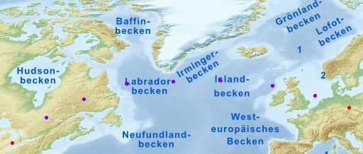
Der Punkt M liegt südöstlich von Kap Farvel (Südspitze von Grönland) etwa auf der Grenze zwischen Labradorbecken und Irmingerbecken.
Die Aufgabe besteht darin, auf der berechneten geodätischen Linie gleichabständige Punkte zu erzeugen und diese in einer Koordinatenliste zusammenzufassen. Der erste Punkt A dieser Liste muss nicht unbedingt der Punkt P sein und der letzte Punkt E dieser Liste muss nicht unbedingt der Punkt Q sein. Statt dessen werden die Punkte über ihre Bogenlängen sA, sE entlang der geodätischen Linie bezogen auf sP = 0 spezifiziert. Der Punkt A=P würde beispielsweise mit sA = 0 adressiert und der Punkt E=Q mit sE = s. Das sind gleichzeitig die Ausfallwerte, wenn keine Bogenlängen spezifiziert werden. Der Mittelpunkt der geodätischen Linie PQ würde beispielsweise mit s/2 adressiert. A oder E dürfen auch außerhalb von PQ, aber nicht extrem weit von P oder Q entfernt liegen.
Weil bisher nur mit ellipsoidischen Längendifferenzen Δλ gearbeitet wurde, benötigen wir außerdem von einem Punkt P oder Q oder A oder E eine absolute ellipsoidische Länge λ.
Die Gleichabständigkeit der Punkte und die Zugehörigkeit zur gewünschten geodätischen Linie kann mit Hilfe von überprüft werden. Seitenlängen und Äquatorazimute müssen für alle Polylinienseiten übereinstimmen. Äquatorazimute müssen auch mit der Vorgabe α0 übereinstimmen. Die Gleichabständigkeit hat eine hohe, aber nicht die höchste Genauigkeit.
Beispiel: Möchten Sie nur die Punkte P und Q in der Koordinatenliste haben, wählen Sie n = 2 als Punktanzahl und lassen Sie die Felder für die Bogenlängen leer.
Die Koordinatenliste besteht aus ellipsoidischen Breiten und Längen. Als ellipsoidischen Höhen wird Null ausgegeben. Die Koordinaten können mit in andere Systemtypen umgewandelt werden.
Die Koordinatenliste kann eines der folgenden Spaltenformate erhalten:
Wir berechnen auf der geodätischen Linie von Dresden (Sachsen) nach Dresden (Ontario) neun gleichabständige Punkte, der ersten Punkt ist Dresden (Sachsen) und der letzte Dresden (Ontario):
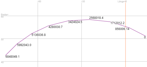
Der fünfte Punkt ist der Mittelpunkt und wird mit φ = 57.77944707385° λ = -39.1962115331° = 320.8037884669° erhalten. Die letzten Ziffern weichen geringfügig vom oben berechneten Mittelpunkt ab, denn wie gesagt, wird die Gleichabständigkeit der Punkte mit hoher, aber nicht immer mit der höchsten Genauigkeit realisiert. Wenn man diese neun Punkte mit berechnet, erhält man zwar ein korrektes und exakt konstantes Äquatorazimut von α0 = 328.3121600°, jedoch differieren die Polylinienseitenlängen um maximal 7 m.
Wir möchten jetzt noch weitere Punkte zwischen den beiden nördlichsten Punkten erzeugen, und zwar im Abstand von 1000 m. Dazu wählen wir die Bogenlängen sA = 2568018.4 m; sE = 3424024.5 m und den Punktabstand Δ = 1000 m.
Wir erhalten 856 Punkte mit tatsächlichen Abständen zwischen Δmin = 1001.1757 m und Δmax = 1001.1768 m. Die Differenz zum gewünschten Wert Δ = 1000 m kommt dadurch zustande, dass die Linienlänge kein ganzzahliges Vielfaches des vorgegebenen Punktabstands ist, so dass der Punktabstand geringfügig angepasst werden musste. Die Äquatorazimute betragen alle exakt α0 = 328.3121600. Der nördlichste Punkt hat eine ellips. Breite von φm = 58.39810555 bei der Bogenlänge φm = 2684154.9. Diese Ergebnisse stimmen exakt mit den oben berechneten Werten für den Grenzparallelkreis überein.
Wenn die Berechnungsaufgabe es wahrscheinlich macht, dass interne Rundungsfehler die Ausgabe verfälschen, wird eine Warnung ausgegeben.
Wenn gegebene Größen nicht fehlerfrei bekannt sind, können Sie berechnen, wie stark sich diese Fehler auf die berechneten Größen fortpflanzen. Siehe hierzu .
Mit dem Rechenwerkzeug kann man auch Meridianbogenlängen berechnen, indem man einfach Δλ = 0 setzt. So erhält man für den Meridianbogen auf dem Bessel-Ellipsoid zwischen den Parallelkreisen φP = 59° und φQ = 60° die Bogenlänge s = 111390.561 m. Mit dem Rechenwerkzeug erhält man denselben Wert, aber mit noch mehr Ziffern: s = 111390.5612847 m
Möchte man nun umgekehrt aus φP = 59°, φQ = 60°, s = 111390.561 m zurück auf Δλ = 0 schließen, ergibt sich keine Lösung. Der Grund ist, dass s abgerundet wurde und somit zu kurz ist. Eine winzige Verlängerung auf s = 111390.562 m schafft Abhilfe und liefert zwei Lösungen Δλ = ±0.00025° ≈ ±0.9''. Geometrisch führen wir hier einen Schnitt von Parallelkreis und ellipsoidischem Kreisbogen aus, der zwei Schnittpunkte ergibt. Diese liegen jeweils etwa 27 m vom gesuchten Meridian entfernt. Grund für die große wahre Abweichung ist die ungünstige Fehlerfortpflanzung, auch als ''schleifender Schnitt'' bezeichnet.
Man konnte diese Situation auch ohne Kenntnis der wahren Lösung erfassen, indem man eine Fortpflanzung des Fehlers in s berechnet. Im folgenden Beispiel nehmen wir einen Maximalfehler von Δs = 0.001 an.
Das ergibt eine Abweichung in Δλ von 0.00011° ≈ 0.4''.
Aufgabe: Wenn Sie auch für φP und φQ Fehlerwerte spezifizieren, erhalten Sie kein Ergebnis. Bitte finden Sie heraus, warum.
|
|
|
|
| Link | Autor(en) | Titel | Jahr | Typ | Seiten MByte |
|---|---|---|---|---|---|
 | Panou G, Korakitis R | Geodesic equations and their numerical solutions in geodetic and Cartesian coordinates on an oblate spheroid | 2017 | GruF | 12 0.1 |
 | Deakin RE, Hunter MN | Geometric Geodesy Part A | 2013 | Lehr | 151 1.1 |
|
| Deakin RE, Hunter MN | Geometric Geodesy Part B | 2010 | Lehr | 212 3.7 |
|
| Deakin RE, Hunter MN | Geodesics on an ellipsoid - Bessel's method | 2009 | Aufs | 66 0.6 |
|
| Deakin RE, Hunter MN | Geodesics on an ellipsoid - Pitman's method | 2007 | Aufs | 19 0.4 |